
Executive Summary
Monte Carlo simulations have become the dominant method for conducting financial planning analyses for clients and are a feature of most comprehensive financial planning software programs. By distilling hundreds of pieces of information into a single number that purports to show the percentage chance that a portfolio will not be depleted over the course of a client’s life, advisors often use this data point as the centerpiece when they present a financial plan. However, a Monte Carlo simulation entails major statistical and philosophical nuances, many of which might be underappreciated by advisors and their clients.
One key nuance to the use of Monte Carlo simulations is whether they are being used as part of a one-time plan versus an ongoing planning process. For example, a Monte Carlo simulation resulting in a 90% probability of success will mean very different things depending on whether a client will take fixed portfolio withdrawals throughout retirement based on the initial probability of success or whether they plan to run additional simulations over time and are willing to adjust their spending based on market performance. For the former client, because a 90% probability of success means that there is a 10% chance they will deplete their portfolio (though the magnitude of the failure is unknown), they might choose to aim for an even higher probability of success to decrease the likelihood that they will run out of money in retirement. But for the latter client, to suggest they have a 10% chance of depleting their portfolio is overstating the risk, as they are willing to adjust their spending in response to future simulations that show a reduced probability of success.
An alternative way to use Monte Carlo simulations for clients who are willing to be flexible with their spending is to consider how spending would change when using a fixed probability of success. For instance, Monte Carlo simulations show that, for any selected fixed probability of success, the maximum and minimum annual spending for a client during the course of their lifetime is remarkably similar. While initial spending levels will be different depending on the target probability of success (as a higher selected probability of success will call for a reduced initial spending amount), adjusted spending levels will track each other closely no matter the initial probability of success chosen. What is different is that those who use a higher constant probability of success will likely have a larger portfolio balance at their death than do clients who choose a lower probability of success at the start of retirement.
This suggests that, in contrast to the view that probability-of-success levels are indicative of the risk of depleting a portfolio, the probability-of-success level used when adjustment is planned for in advance is essentially akin to putting your thumb on the scale to slightly favor either maintaining current income (lower probability of success) or preserving estate balance (higher probability of success). In other words, if an advisor is going to use Monte Carlo on an ongoing basis, then the probability of success threshold targeted is more akin to a slider that adjusts the degree of preference for current income or legacy rather than a meaningful measure of the likelihood of depleting a portfolio.
Ultimately, the key point is that because the results of Monte Carlo simulations contain a significant amount of nuance, particularly if being utilized as part of an ongoing planning relationship, advisors can consider using them as an internal analytical tool but communicating the results through the use of risk-based guardrails or as a tradeoff between current income or legacy interests to help clients better understand what the results actually mean for their financial plan!

Monte Carlo simulations have become the dominant method for conducting financial planning analyses for clients, and most fully fledged financial planning software today includes the ability to conduct Monte Carlo analyses. Some specialized tools in areas such as Social Security planning even include capabilities for Monte Carlo simulation.
Nonetheless, as an industry, we are still in the infancy of using and understanding Monte Carlo analyses for clients. While some Monte Carlo simulators have become so simple to use that they can be easy to overlook, the reality is that there are some major statistical and philosophical nuances that go into using Monte Carlo simulation, some of which continue to be underappreciated by financial advisors.
For instance, while a recent experimental survey found that financial advisors recommend the same probability-of-success thresholds when conducting one-time and ongoing financial planning projections, the reality is that risk levels associated with the same probability-of-success threshold are very different when considered in the context of a one-time plan versus part of an ongoing financial planning service provided to clients.
Why One-Time Projections Are Different From Ongoing Plans
While it can be easy to gloss over, there is a major difference between Monte Carlo simulations used as part of a one-time plan versus an ongoing planning process.
Monte Carlo Simulations For One-Time Plans
Let’s first consider what Monte Carlo means in the context of a one-time plan.
Example 1. Suppose John is 65 and has hired a financial advisor to run a one-time projection for him. He wants to determine how much he can afford to spend in retirement but would like to manage his investments himself and is not interested in a long-term relationship.
John’s advisor runs a plan based on John’s current assets and desired spending level, which results in a 90% probability of success. John is satisfied with this result and decides he will enter retirement spending at his desired level based on this one-time analysis.
Let’s first take some time to really think about what the projection for John in the example above is saying in this case. Based on the assumptions used (i.e., John’s current assets and desired spending level), John’s projected spending would have resulted in depleting his portfolio 10% of the time. Notably, this says nothing about the magnitude of failure (and that is a major limitation of Monte Carlo simulation as commonly used currently). We haven’t specified what John’s guaranteed income levels are and, therefore, we can’t say whether spending down the rest of his assets is a financial catastrophe or perhaps just a minor inconvenience. Nonetheless, setting that concern aside, let’s continue to look at exactly what this result is saying.
Another important assumption here is that John isn’t going to concern himself with what goes on in the markets going forward – as a one-time projection would presume. He’ll continue to charge forward blindly spending according to the initial plan. What we know from the outset is that there will be a wide range of possible long-term outcomes for John. Under some scenarios, John will experience a favorable sequence of returns and he’ll accumulate substantial sums of money – potentially far more than he might optimally be targeting. Notably, the ability to adjust is a powerful tool that John has at his disposal, but since we are considering the case of using Monte Carlo for a one-time plan, we’re going to presume that John is comfortable with the 10% chance of depleting his portfolio and doesn’t wish to revise his spending level.
Notably, while John will not be updating his Monte Carlo simulation over time, if he were to update the assumptions used in his plan, we would expect from the outset that the probability of success level would change dramatically over time (and based on actual returns experienced). A 90% probability of success only applies to John’s plan at this moment in time, but that risk level would change in either a positive or negative direction as John experiences market returns.
One of the most important implications for the use of Monte Carlo in a one-time plan is that only doing a one-time plan comes with significant risk. With this one-and-done approach, there’s no refinement or adjustment. As a result, individuals using a one-time approach might want to be extra careful in selecting a probability of success level.
In John’s case above, is he really comfortable with a 90% probability of success? If he’s not going to adjust his spending level, would it be worth increasing the probability of success to 95%? We can’t answer these questions since the answers ultimately come down to John’s risk tolerance (which is unknown in this example) and are also likely influenced by his magnitude of failure (which is also unknown), but, the key point here is that John will want to be very careful in selecting this probability-of-success level for his one-time plan. As we’ll see in the next section, the dynamics for ongoing planning are actually very different.
It is worth noting that this one-time planning approach to Monte Carlo simulation is likely used by few, if any, advisors. Even project or hourly planners generally recommend that clients come back for plan updates, so this likely feels like a bit of a foreign concept when described this way.
Nonetheless, the probability-of-success metric so widely touted by almost all Monte Carlo software is actually a reflection of risk in precisely this context. Monte Carlo simulations, as commonly practiced today, are almost always answering the question, “Given the information we have at this moment in time, if you charged forward blindly for the next X years following the defined spending pattern, what percentage of the time are we simulating you would deplete your portfolio?”. The probability-of-success metric so widely touted actually gets substantially less intelligible when interpreted in an ongoing planning context.
Monte Carlo Simulation For Ongoing Plans
Although most advisors use Monte Carlo simulation in an ongoing manner, the interpretation of probability-of-success results in the context of an ongoing plan actually gets a bit more abstract and harder to understand.
Example 2. Suppose Sarah is 65 and has hired a financial advisor to provide ongoing financial planning services for her, including ongoing updates to her retirement projections. She wants to determine how much she can afford to spend in retirement now, and what it would require to stay on top of opportunities to adjust her spending if warranted.
Sarah’s advisor runs a plan based on Sarah’s current assets and desired spending level, which results in a 90% probability of success. Sarah is satisfied with this result and decides she will enter retirement spending at her desired level. However, Sarah is also open to adjusting her spending as warranted.
Notably, assuming that the plans for John (from Example 1, earlier) and Sarah (from Example 2, above) were otherwise identical, this first plan that was created for the two of them would be identical. However, the risk associated with a 90% probability-of-success threshold is now quite different for Sarah, who plans to revisit her plan and potentially adjust her spending if needed.
We’re reporting a 90% probability of success metric that assumes charging forward blindly despite knowing that Sarah has no desire to charge forward blindly. Therefore, to suggest that Sarah has a 10% chance of depleting her portfolio is overstating her risk. This was perfectly accurate for John, who did not plan to adjust his spending, but it is not accurate at all for Sarah, who plans to make adjustments as needed.
That’s not to say that this risk level at a given point in time is a useless metric for Sarah, but hopefully this helps draw some attention to why a 90% probability-of-success level is very different in these 2 cases. We know from the outset that downside risk is overstated for Sarah despite it not being overstated for John.
Let’s suppose John and Sarah both retire at the same time and catch a bad sequence of returns at the start of retirement. Furthermore, let’s assume that re-running their plans at this time would result in a 70% probability of success for each of them. In John’s case, he doesn’t care. Probability of success could drop to 1% and he’s still not going to change his spending. But Sarah had planned to make adjustments as needed. At some point, with the guidance of her advisor, she would cut back on spending.
Let’s suppose Sarah and her advisor decide now is the time to reduce her spending and Sarah makes adjustments to get her back to what would be a 90% probability of success. Sarah has made a significant alteration to a scenario that the Monte Carlo simulation was suggesting still had a 7-out-of-10 chance of not depleting her portfolio.
Whether that is the ‘right’ level to adjust will again depend on Sarah’s risk tolerance, magnitude of failure, etc. However, what we can say is that the original 90% result makes little sense in light of her now subsequent reduction. Likewise, even the 70% and 90% results from the updated analysis again aren’t particularly accurate reflections of her real chances of depleting her portfolio when she knows in advance that she plans to make spending adjustments.
Again, while the probability-of-success metric is still useful for understanding momentary risk levels, it is really quite off in terms of expressing the likelihood that someone who plans to make spending adjustments along the way would actually deplete their portfolio.
What Is Monte Carlo In An Ongoing Context?
If probability of success isn’t really an accurate reflection of the risk of depleting a portfolio, then what is it, exactly? Monte Carlo remains a useful metric for understanding momentary risk levels as they relate to one another, but it really doesn’t speak to long-term risk in a meaningful way.
Although we allowed Sarah’s probability of success to drift from 90% to 70% in Example 2 above, let’s consider a different strategy she could make to adjustments: continually updating her spending to maintain a target momentary risk level.
Notably, this is not a very practical strategy. It’s doubtful that any client would want such volatile spending, but it is still a useful scenario to consider for illustration purposes:
Example 3. Everything about Sarah’s scenario remains the same as above in Example 2, except now she wants to target a constant 90% probability-of-success level.
If Sarah is trying to target a 90% probability of success on a continual basis, then her 90% probability-of-success spending level is going to fluctuate up and down with the market.
While this again isn’t a particularly practical approach to go about spending, it’s an approach that is useful for gaining a better understanding of what “probability of success” is really getting at in an ongoing planning context.
Consider some results from a prior analysis where we compared spending levels at a 95% constant probability of success, 70% constant probability of success, 50% constant probability of success, and 20% constant probability of success.
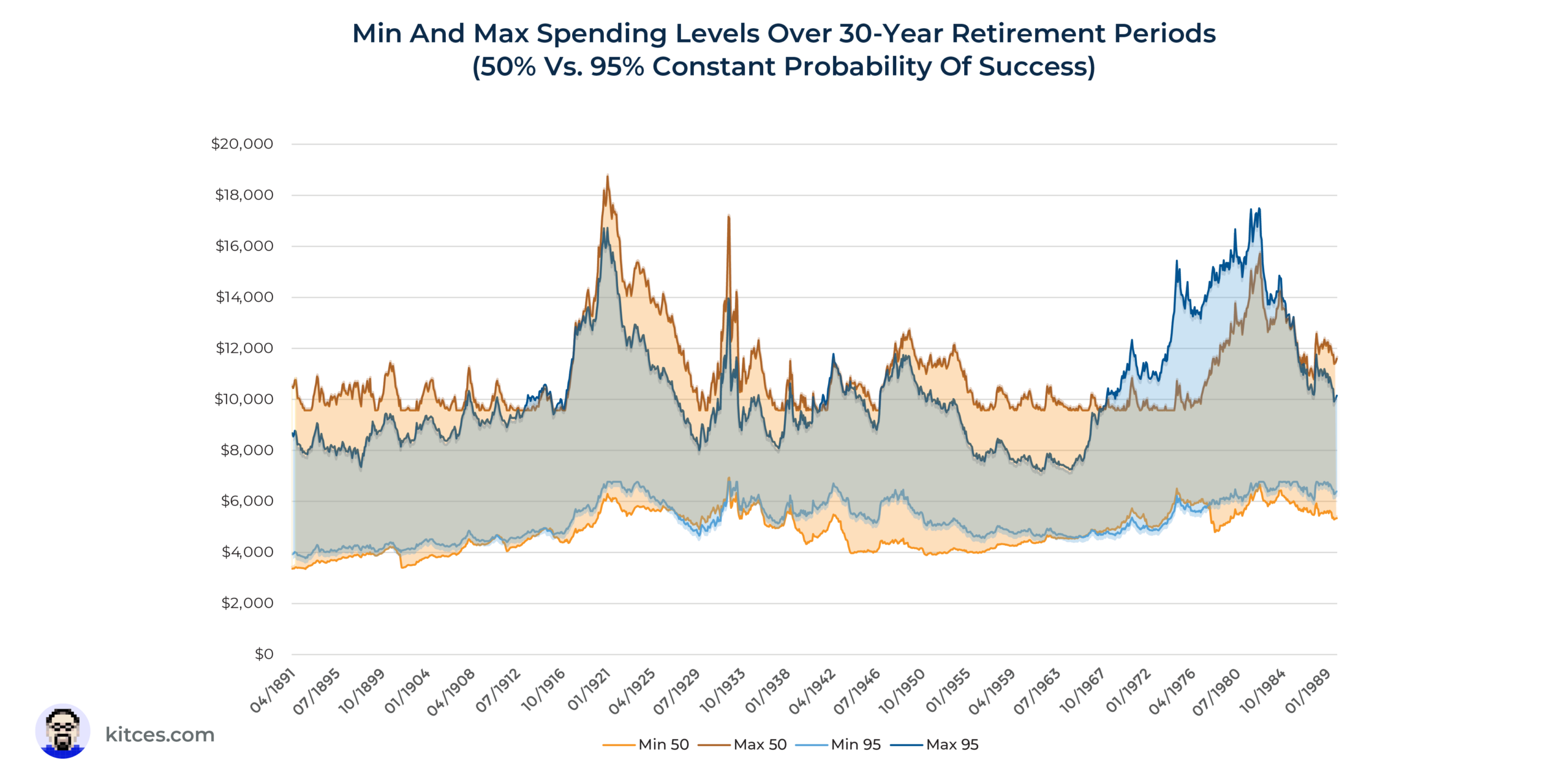
First, to look at the 95% probability of success threshold, consider the following graphic which shows the range of inflation-adjusted spending levels over 30-year retirement periods beginning on the dates shown on the x-axis.

What the chart above is saying is that, based on the plan analyzed (again, see here for more detailed assumptions) for the 30-year retirement period beginning in April of 1891, inflation-adjusted spending levels for someone following a constant 95% probability of success spending strategy would have ranged from about $4,000 per month to roughly $8,500 per month. To calculate this, we are combining historical analysis with Monte Carlo simulation. We are starting someone at a given point in history, using a Monte Carlo simulation to determine their 95% probability of success spending level, then stepping them forward one period in history based on actual returns experienced and then updating their Monte Carlo plan and solving for their new 95% probability of success spending level.
Notably, inflation-adjusted spending in the constant 95% probability of success scenario during the 30-year period beginning in April of 1981 above would have started out around $6,800 per month, so there were both increases and decreases.
Now, let’s repeat the same process but add in the spending ranges for someone planning to a constant 50% probability of success:

While I’ve previously written about these same results in greater detail, what’s striking about them is how consistent the range of spending was regardless of whether the individuals here planned to a constant 95% probability of success or a constant 50% probability of success (and, in fact, the same even holds at a 20% probability of success!).
Why? Because momentary probability of success is not a very intelligible concept when change is planned for from the outset, even to advisors who likely understand Monte Carlo simulation significantly better than most people.
Unlike the one-time plan where a lower probability-of-success level does meaningfully influence the risk of depleting a portfolio, lower probability-of-success levels have a trivial impact on the risk of depleting a portfolio if adjustments will be made going forward.
What we’re seeing in the chart above is essentially a reflection of the fact that, for someone who plans to use Monte Carlo on an ongoing basis, the market is going to drive spending outcomes far more than the probability-of-success threshold chosen. Granted, this does not necessarily apply to initial spending levels, as those will be significantly higher with lower probability of success scenarios, but adjusted spending levels will track each other directionally up and down over time.
Instead, the probability-of-success level used is essentially akin to putting your thumb on the scale to slightly favor either maintaining current income (by choosing a lower probability of success) or preserving estate balance (by choosing a higher probability of success). In other words, if an advisor is going to use Monte Carlo on an ongoing basis, then the probability of success threshold targeted is more akin to a slider that adjusts the degree of preference for current income or legacy rather than a meaningful measure of the likelihood of depleting a portfolio.

Monte Carlo Simulation As Part Of An Ongoing Service
As noted previously, few advisors are running Monte Carlo simulations intended as truly one-time projections. Even project-based planners who don’t work with clients on an ongoing basis will generally recommend getting plans updated periodically.
But this draws attention to an interesting disconnect between how advisors commonly think of probability-of-success thresholds. According to the common view, probability-of-success thresholds tell us something about the likelihood of depleting a portfolio at a given spending level. However, recall that this is only true for one-time projections that will not experience spending adjustments.
If plans will be adjusted on an ongoing basis, though, then the accurate view is that a probability-of-success threshold is really just setting a preference somewhere on a spectrum from a high preference for maintaining current income (low probability of success) to a high preference for preserving legacy assets (high probability of success).
Yet, it appears that this understanding of the distinction between Monte Carlo in a one-time-plan context and Monte Carlo in an ongoing planning context is not well appreciated. Recall that an experimental study found that advisors expressed no difference in probability-of-success thresholds targeted regardless of whether they were asked to provide a threshold for a one-time plan or an ongoing plan.
This is all particularly important since the way many of us think about probability of success (i.e., as the risk of depleting a portfolio) is actually inaccurate for the ways that we use Monte Carlo with clients.
Ultimately, this is likely good news for further demonstrating the value of financial planning as an ongoing service. Ongoing updates to a financial plan are very important. Additionally, it turns out the key metric spit out by Monte Carlo software means something very different depending on whether you are using Monte Carlo for one-time plans versus ongoing planning.
This is a level of nuance that will likely be missed by almost all DIY retirement planners. However, trying to explain to clients why probability of success is not a measure of the risk of portfolio depletion in an ongoing planning engagement requires a level of depth in understanding Monte Carlo simulation that most clients will not have, and therefore will likely not be a successful endeavor.
And the futileness of explaining to clients what probability of success actually means in an ongoing context is yet one more reason why perhaps probability-of-success metrics should really be pushed ‘behind the scenes’ as an important technical nuance for advisors to understand but that rarely actually gets reported to clients – similar to how doctors are going to know all sorts of technical details about how to read an EKG that never gets reported to patients.
Risk-based guardrails (expressed in dollar terms) including probability-of-success-driven guardrails are one such alternative presentation of Monte Carlo results that avoid these issues. Rather than talk about confusing probability-of-success thresholds, Monte Carlo results can instead be presented in terms of current spending levels, portfolio balances that would trigger a spending change, and dollar amounts of spending changes if a change was triggered.
These are practical results that rely on language (income/spending adjustments/dollars) that clients can actually understand. Moreover, guardrails provide actionable advice that can actually help orient behavior – not to mention the peace of mind that can come from knowing what will happen ahead of time.
If all a client knows is that their spending level reflected a 90% probability of success before a downturn started, then they’re likely going to be quite stressed as they watch a $2 million portfolio fall to $1.6 million. However, if they knew in advance that, for their particular plan, their portfolio would need to fall to $1.4 million before a spending adjustment would be triggered (and that at that point the trigger would only be a $300/month reduction in spending), then that can be incredibly powerful information for calming a client in the midst of a tumultuous market.
Consistent with the theme of removing the focus from probability of success, software companies may want to consider an option to remove probability of success entirely as a focal point, and instead build in something like a slider that would more accurately ask an advisor/client to define the desired preference for current income versus legacy assets.
Because, ultimately, that is what probability-of-success thresholds are actually getting at in an ongoing context, even if most advisors mistakenly think of probability of success as if it were being used in a one-time plan, instead.

