
Executive Summary
Financial advisors often use Monte Carlo simulation in their financial planning process, which (as is commonly found in major financial planning software packages) traditionally presents the results of the projection in terms of probability of success or failure (with ‘success’ being defined as an iteration of the plan where the client doesn’t run out of money, and ‘failure’ signifying the opposite).
However, some commentators have taken issue with this framing, particularly as it concerns the way that Monte Carlo results are presented to clients. Most significantly, the ‘success/failure’ framing fails to capture the reality that retirees, when facing an unlucky sequence-of-returns scenario which could result in their running out of money, can and often do make adjustments to their spending that allow them to avoid that unfortunate outcome.
To better reflect this reality, the phrase “probability of adjustment” has emerged as a commonly suggested alternative to “probability of success”. While representing an improvement over the original, however, “probability of adjustment” itself can be prone to ambiguity and misinterpretation without being clear about what type of adjustment might be needed, and what the outcome might be if that adjustment weren’t made.
A Monte Carlo simulation can tell us, with the benefit of hindsight, exactly which iterations of a plan would have ended with the retiree running out of money. But in reality, retirees do not have the ability to know which iteration (if any) they are on, and in many instances will likely make adjustments in cases where, in hindsight, no adjustment was strictly necessary. As a result, simply replacing “probability of success” with “probability of adjustment” when communicating Monte Carlo results can significantly underestimate the likelihood that a client will actually make an adjustment at some point, since clients (and advisors) do not have the benefit of knowing when an adjustment is ‘truly’ necessary.
Likewise, if an advisor were to recommend a dynamic spending strategy based on Monte Carlo simulations (such as adjusting spending to maintain a constant probability-of-success level), the “probability of adjustment” framing can skew even further from reality, since preserving a consistent probability of success often calls for relatively frequent adjustments in spending. For instance, maintaining a 70% probability of success level – implying only a 30% probability of adjustment – would in reality have required downward spending adjustments in nearly 100% of all historical scenarios, which would understandably have caused confusion for many clients if the advisor had used the standard “probability of success/adjustment” framing!
Ultimately, the key point is that outcomes, not probabilities, are what matter to clients, and any way of communicating Monte Carlo results should be clear about what those results mean in terms of real spending to the client. Though “probability of adjustment” is an improvement over “probability of failure”, it can still greatly underestimate the probability of actual spending adjustments, especially when dynamic spending strategies are involved. In those cases, it may make sense to avoid framing Monte Carlo results in terms of probabilities entirely, but rather to communicate in terms of the actual dollar spending adjustments that would be triggered in specific scenarios – which is what really matters to the client in the end.

Many articles have noted a number of communication disadvantages associated with using “probability of success” to report Monte Carlo results. For instance, our brains may struggle to understand how to interpret probabilistic results, the implication of ‘failure’ in retirement may exacerbate client fears, clients may succumb to the ‘wrong side of maybe’ fallacy and judge advisors more harshly than they should when difficult sequences of returns are encountered, among others.
A major issue with the success/failure framing is that it is overly binary and fails to capture the reality that retirees can adjust when needed, and that it often only takes small spending adjustments to keep a plan on track. As a result, it has been suggested that a ‘probability of adjustment’ framework, instead of one based on ‘probability of success’, may better convey the actual consequences for retirees.
Furthermore, some experimental research has even found that there are a number of advantages to adjustment-framing over success-framing when it comes to reporting Monte Carlo results, including improved client emotional responses, a better understanding of plan results, and even improved perceptions of advisors themselves.
And yet, while there are advantages to framing results about probability of adjustment rather than probability of success, there are easily misunderstood aspects of ‘probability of adjustment’ that can lead to confusion among both advisors and clients.
The Dual Meanings Of “Probability Of Adjustment”
At the heart of potential misunderstandings around what probability of adjustment means is that there are two equally valid ways that one might interpret the phrase:
- Probability that downward adjustment would have been needed to avoid depleting a portfolio.
- Probability that downward adjustment would have been triggered using a dynamic strategy.
The phrase ‘probability of adjustment’ is itself ambiguous, and it is easy to see how one might even mistakenly conclude that the two interpretations above are essentially the same (or at least similar enough). However, the reality is that these are extremely different concepts, and only one is synonymous with “probability of success” in a Monte Carlo simulation.
First Meaning: Downward Adjustment Needed To Avoid Depleting A Portfolio
First, consider the probability that a downward spending adjustment would have been needed to avoid depleting a portfolio. This metric is synonymous with the traditional probability of success metric that dominates Monte Carlo simulation.
Here, we are effectively saying, “If we look back after the fact, what percentage of the time was a portfolio depleted?” Since these were the only iterations within the Monte Carlo simulation that actually ran out of money, then, at the same time, these were the scenarios that were ‘failures’ by traditional reporting.
Notably, this portfolio-depletion perspective is an entirely after-the-fact metric. It does not encompass the totality of cases where someone using a dynamic spending strategy would have made an adjustment, and that’s where the confusion can arise.
For example, suppose Jessica is a financial advisor who is running a Monte Carlo simulation and receives a 90% probability of success result for her client. Jessica has read some about the benefits of using probability of adjustment in lieu of probability of success, and therefore tells her client:
Using the strategy we have outlined here, the results of our analysis suggest that there’s a 10% chance you would need to make an adjustment by reducing your spending in the future to avoid running out of money.
That might seem right if someone is thinking about using ‘adjustment’ in lieu of ‘success’ (or, more precisely, failure), but this is not quite right and, unfortunately, could paint a wildly inaccurate picture for Jessica’s client.
A more accurate reporting might have been something along the lines of the following (where, for the sake of argument, we are assuming that ‘failure’ is defined as depleting the portfolio, although certainly some other targeted estate balance could be used):
Using the strategy we have outlined here, the results of our analysis suggest in about 10% of simulated cases a downward spending adjustment would have been needed to avoid completely depleting a portfolio.
This might seem like splitting hairs, but the differences here are actually very significant. The major risk here is that the client could walk away thinking that there is only a roughly 1-in-10 chance that they would need to reduce their spending in the future using a dynamic strategy, but this would be way off the mark (as we’ll take a look at later), since the reality is that there are many instances when a prudent individual who doesn’t have the benefit of hindsight would have made adjustments that they ultimately did not need to be made.
Second Meaning: Downward Adjustment Triggered Using A Dynamic Strategy
Second, let’s consider ‘probability of adjustment’ as the probability that a downward adjustment would have been triggered using a dynamic strategy.
This is the meaning of adjustment that is actually analogous to the likelihood of needing to make a future downward spending adjustment and, as mentioned above, is a far different concept than the after-the-fact view of how many scenarios did fully run out of money.
In this case, we don’t have the benefit of hindsight. Suppose Jessica’s client, from the earlier example, starts her journey and hits a terrible initial sequence of returns, and her probability of success falls all the way to 50% only 5 years into her plan.
Would it be prudent for her to make an adjustment? Most advisors would likely agree that it would be, as the odds that she does end up depleting her portfolio are higher than many might feel comfortable with. However, note that even at this point, what the Monte Carlo results are telling us is that 1-out-of-2 times, we would expect that she wouldn’t need to make a downward adjustment.
In other words, while the prudent thing to do here may be for Jessica’s client not to roll the dice and hope that she ends up with the 1-out-of-2 outcome (i.e., she should make an adjustment now to more prudently manage her risk), the reality is that in a non-trivial number of Monte Carlo iterations Jessica was not depleting her portfolio despite the bleak outlook.
Let’s suppose Jessica was in one of the 1-out-of-20 scenarios that would have turned out fine, but that she made an adjustment anyway. Essentially, this is a ‘false positive’ result where a spending reduction is a prudent action, even though it ended up not being called for. Furthermore, note that such false positives will likely occur even at higher probability-of-success levels, such as 10%, 50%, 70% (as one prior study found that many advisors treat 70% as a minimally acceptable threshold for ongoing planning success levels), and higher.
Or, to put it simply, sometimes it’s prudent to make adjustments even when we would find out after the fact that it ended up not being necessary to do so.
Anecdotally, this seems to be what a non-trivial number of advisors intuit or presume the ‘probability of adjustment’ is telling them. Unfortunately, that belief can lead advisors (and their clients) wildly astray.
How Different Are The Two Ways Of Thinking About Probability Of Adjustment?
At this point, it is reasonable to wonder how different these two concepts – namely, the consideration of probability of adjustment as a need to avoid portfolio depletion, versus a trigger set in place by a dynamic strategy – really are if we were to quantify them.
For instance, if it’s true that false positives occur but that they only occur very rarely, then maybe this is all much ado about nothing. Perhaps a 5% chance of future downward adjustment becomes a 7% chance of future downward adjustment, and, at that point, do we really care? Most people probably struggle to make a discernable distinction between 5% and 7% anyway, so the harm may be minimal if we are still getting roughly the same idea conveyed even if the numbers are slightly different.
On the other hand, if it turned out that 90% of the time people using a dynamic plan experienced a downward adjustment even when starting at a 95% probability of success, then it likely wouldn’t be wise to set expectations poorly by framing the outcome as only having a 5% chance of future downward adjustment.
To test whether false positives using a dynamic spending strategy are something we need to be mindful of, we can use a combination of historical simulation and point-in-time Monte Carlo calculations while we walk individuals through historical sequences. For this particular analysis, we’ll examine several strategies that hold probability-of-success levels constant. For instance, if we are examining a constant 95% probability-of-success level, then we use Monte Carlo to set the spending level where it would be based on the assumed starting point, then step an individual forward one month in the historical sequence we are examining based on what actually happened in the market, and then recalculate their new spending level that would maintain a 95% probability of success based on distributions they took and what has happened in the market.
We’ll be using 30-year retirement periods and repeating this process for each 30-year sequence from 1871 to the present (see here for a fuller explanation of the methodology used here).

Nerd Note:
From a statistical perspective, it would be ideal to use an in-sample approach and change capital market assumptions based on the information that one actually had available to them at each point in history as it unfolded, so that we aren’t ‘cheating’ by giving someone access to data they would otherwise not have. However, for simplicity, we have used a single out-of-sample set of capital market assumptions based on historical averages over the entire time period.
For this analysis, it is also important to define what we mean by a “downward adjustment.” One approach could be to use any downward adjustment, and while that is a defensible definition, it won’t provide a tremendously insightful analysis because even a single down period in an entire 30-year sequence would, by definition, result in a downward adjustment.
Instead, we will be defining a downward adjustment as a spending reduction relative to an inflation-adjusted initial spending level. In other words, we consider an adjustment to be downward if someone actually has to cut back to below where they initially started spending in real dollars.
As an example, suppose John starts spending at $8,000 per month (at a 95% probability of success level). His spending goes up to $10,000 per month as the market rises (and, therefore, the level of spending to maintain a 95% probability of success has gone up as well). However, the market later pulls back and John’s new 95% probability-of-success monthly spending level goes down from $10,000 to $8,500. In this case, we aren’t considering this to be “downward adjustment” since the adjustment was not down overall relative to the initial real spending level of $8,000.
However, suppose that, to maintain a constant 95% probability of success, John’s spending starts at $8,000, goes up to $10,000, and then falls to $7,900 (all adjusted for inflation). In this case, we would consider it a downward adjustment, because now John’s new spending level of $7,900 is less than his initial spending of $8,000 in real dollars.
Furthermore, we would still consider this a historical sequence that experienced a downward adjustment even if John’s spending subsequently rose above $8,000 in real spending and never saw another reduction below $8,000 throughout the entire 30-year-sequence.
To examine this more closely, let’s consider a scenario involving a hypothetical client:
- Hank (66) and Marie (64) are married.
- They have $1 million invested in a 60/40 portfolio.
- They pay 1.2% in all-in weighted average fees.
- Their combined monthly income is $3,500 in Social Security.
Furthermore, we assume the following:
- They want to leave a $200,000 (adjusted for inflation) legacy to their children.
- They are willing to make adjustments to their spending and do so for whatever adjustment is necessary each month. (Note: To keep assumptions simple, adjustments are made monthly no matter how small the adjustment, but obviously in the real world there would probably be more lag with slightly fewer but potentially larger adjustments, such as reviewing and potentially adjusting spending at each annual review meeting).
Let’s start by considering a scenario where Hank and Marie aim to maintain a constant 20% probability of success. Not surprisingly, this level is quite aggressive, and downward adjustments are very common, occurring in 100% of historical sequences.
Likewise, a constant 50% probability of success also saw downward (real) adjustments 100% of the time.
However, both of the probability of success thresholds above are not commonly used among advisors (despite 50% probability of success not actually being as bad of a target as commonly believed, especially for advisors who are doing ongoing planning rather than one-time planning), so how would the same analysis fare as we start to get into higher, more commonly used probability of success levels?
At a constant 70% probability of success – roughly the minimum that advisors have reported in prior studies being comfortable using – we still see very high adjustment rates at 99.57% of the time. In other words, despite only 30% of scenarios ultimately running out of money if no adjustments were made, we still see that proactive adjustments were called for in 99.57% of historical scenarios when planning to a constant 70% probability of success!
And this is important, because if an advisor is trying to set expectations by telling their client that the client only has a 30% probability of needing to adjust their spending – when the reality is that 99.57% of the time, historically, they would have had to adjust spending when looking forward proactively – then that presents a very major opportunity for setting expectations poorly!
And even if we bump the constant probability of success level all the way up to 95%, we still see that about 96.3% of plan scenarios experienced a downward adjustment when planning proactively! In other words, even though only 5% of iterations modeled resulted in fully depleting a portfolio, it was still the case that over 96% of iterations modeled experienced some reduction in real spending throughout the full retirement sequence – suggesting that describing a 95% probability of success as having a 5% “probability of adjustment” could be wildly misinterpreted.

What About Big Downward Adjustments?
While the numbers above might be surprising, it is certainly true that in some of these cases the downward adjustments may have been trivial. For instance, as described above, even a reduction of $1 in monthly income would result in a sequence that has a downward adjustment, when, in reality, that’s really not a meaningful downward adjustment from a practical perspective.
But what if we use something more substantial to define a downward adjustment? Say, 35% less (adjusted for inflation) than initial spending levels?
In this case, using the same 20%, 50%, 70%, and 95% probability of success thresholds, we see the following results:

While the numbers here are less extreme, they still go a long way toward highlighting the risk of telling someone that they only have, say, a 5% probability of a downward adjustment could lead to a lot of confusion. Even when using a 95% constant probability of success, a full 15% of the time saw reductions of 35% or more!
How Advisors Can Communicate Monte Carlo Results
Ultimately, the key takeaway here is that referring to the “probability of adjustment” as the probability that downward adjustment is needed to avoid portfolio depletion is not the same thing as referring to it as the probability that downward adjustment is called for in a dynamic retirement spending approach. This is an important distinction, because “probability of adjustment” is ambiguous and arguably could refer to either one of these, when the reality is that only the former is actually synonymous with “probability of success” from a Monte Carlo simulation.
And, as noted above, we see that dynamic strategies do often call for reductions at some point in time. Even when starting out at a 95% probability of success level (and maintaining that throughout the plan), we still saw real reductions in spending in as many as 96% of scenarios.
Granted, planning to a constant probability of success is likely not a wise thing to be doing in the first place. We should expect that, as the market ebbs and flows, probability of success levels will rise and fall accordingly. Building in some buffers before making adjustments could help avoid both increases and decreases that are simply the result of short-term noise in the market. But where should a spending decrease be triggered? 70% probability of success? 50% probability of success? Even lower?
While some further work in this area is still needed, it is worth noting that trigger points below 50% probability of success are not as outlandish as some might think when used as part of an ongoing planning process. In fact, trigger points of 40%, 30%, or even 20% probability of success might be reasonable as part of an ongoing planning strategy, and even planning to a constant 20% probability of success results in far fewer differences than planning to a constant 95% probability of success than most might think.
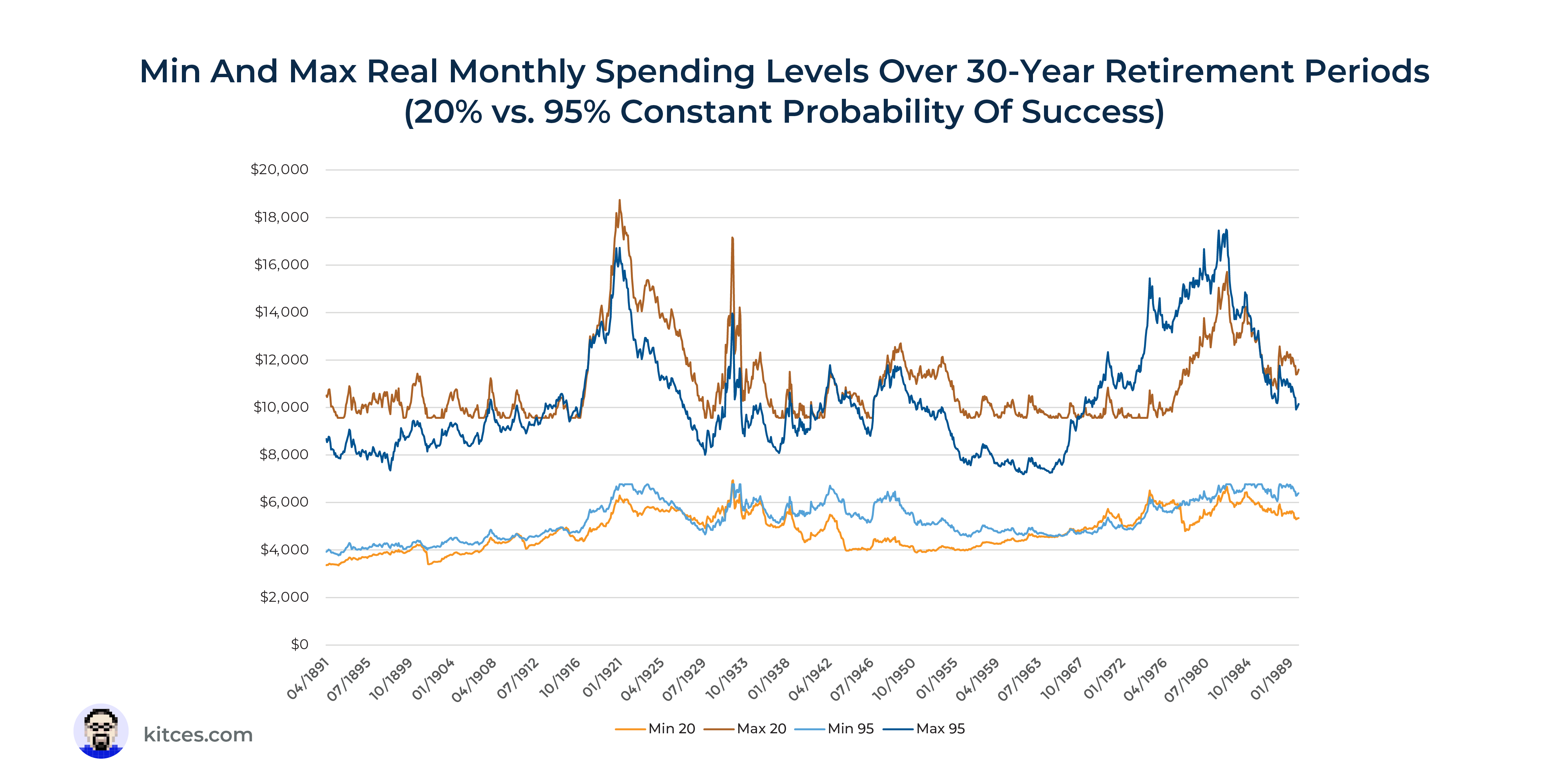
For instance, see the chart below that summarizes the differences in maximum and minimum spending levels over 30-year sequences when planning to a constant 95% probability of success versus a constant 20% probability of success:

What’s particularly striking about these results is how similar spending levels are between probability of success levels held constant at both 95% and 50%. In other words, even if a retiree accepts a 50% probability of success, as long as they’re willing to make the adjustments along the way, the minimum and maximum spending levels are still quite similar!
Of course, as discussed in our earlier article, the caveat is that for the retiree who starts with a lower probability of success and a higher initial spending level, falling to a ‘similar’ minimum spending level will still reflect a much bigger relative cut in spending from where their retirement started and will be a bigger adjustment to handle.
Total Risk Guardrails Offer Better Communication Focal Points
When thinking about how to describe probability of adjustment to clients, it is also worth considering whether it really belongs as a focal point in the first place. As we’ve covered here, there’s a lot of risk of confusion associated with the use of probability of adjustment, even if it is superior to probability of success.
An approach like total risk guardrails might instead provide much better dynamics for actually communicating results that matter. For instance, we could have a total risk-based guardrails plan that looks something like the one below:

Here, we are still using probability of success as a key metric for setting these initial spending levels and guardrails, but the results are presented at a much better level of abstraction for the client by focusing on what actually matters to them more.
Instead of simply saying, “Mr. and Mrs. Client, our analysis suggests you can spend $52,000 per year now. This plan was run at a level of only needing to make an adjustment to avoid depleting your portfolio in about 5% of scenarios considered,” clients are being given specific guidelines for when a reduction would be called for in terms of actual dollars.
For instance, “Mr. and Mrs. Client, your portfolio is currently at $1 million and we would suggest that you can spend about $52,000 per year. However, if your portfolio falls to $740,000, then we would suggest cutting your income back to $48,500, which is about $300 per month.” Of course, this is also an opportunity to note the upside potential that would come from increasing spending close to $14,000 (from $51,900 to $65,800) if the portfolio were to increase in value by $270,000.
Ultimately, this is far more practical for the client, even though advisors could be running the plan with the exact same software and using the exact same probability of success levels (see here for a fuller explanation of how typical Monte Carlo software could be used to generate probability-of-success-driven guardrails).
The key point is that communicating results from a guardrails-based plan in terms of dollars to clients is likely far more effective for communication than reporting a probability of adjustment metric, given the ambiguity and confusion that exists around that term itself. So, despite the real advantages of talking in terms of probability of adjustment rather than probability of success, making that shift may only be one small step toward even better ways to focus on and report plan results for clients.
For more client communication strategies related to retirement planning, join Derek for his upcoming webinar, Improving Monte Carlo In Retirement Planning: Best Practices For Better Conversations, on July 5th. More information is available here.

